
 Support Center
Use Case Tutorial:
3D Depth from Surface Normals using a Polarization Camera
Shape-from-Polarization (SfP)
This document will discuss how to inspect the 3D geometric structure of an object from surface normals by using a polarization camera. The Phoenix and Triton polarization cameras can be used to analyze the polarization state (AoLP, DoLP, and Intensity) of the light reflected from an object to estimate surface normals. Surface normals that are out of tolerance or vastly different from their neighboring normals can be treated as defects and deformations in the object, such as a dent in a metal can. In addition, the surface normals can also be used to reconstruct a 3D point cloud of the target object. This technique is useful in analyzing object shape quality if one does not have access to a 3D depth camera.
Requirements:
- Triton (TRI050S-P/Q) or Phoenix (PHX050S-P/Q) 5.0 MP polarization camera
- Appropriate lens for your setup (Fujinon C-Mount 5MP 2/3″ 8mm f/1.6)
- Unpolarized light source (SCHOTT EasyLED Spot Light, Edmund Optics #15-921)
- Arena SDK (Use ArenaView to capture polarized image)
- Matlab 2020b or GNU Octave 4.4.1
Deformation Example using Dented Metal Can
Showing Deformation
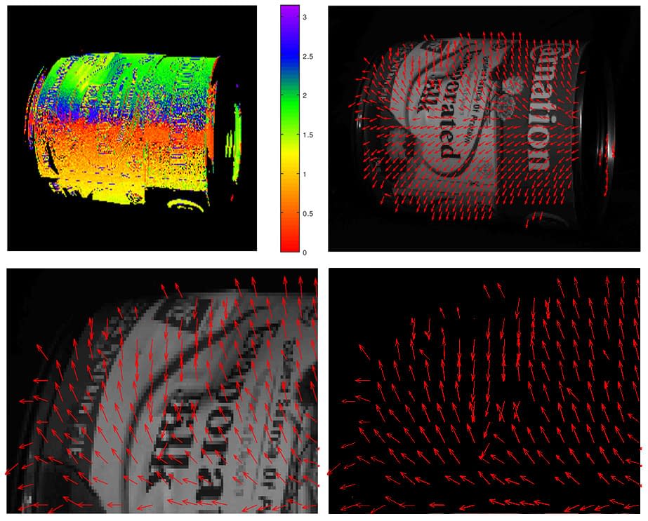
The images below show how surface normals (red arrows) can be used to identify deformation in an object’s shape. The dent can be seen with surface normals pointing in very different directions than surrounding normals.
No Deformation
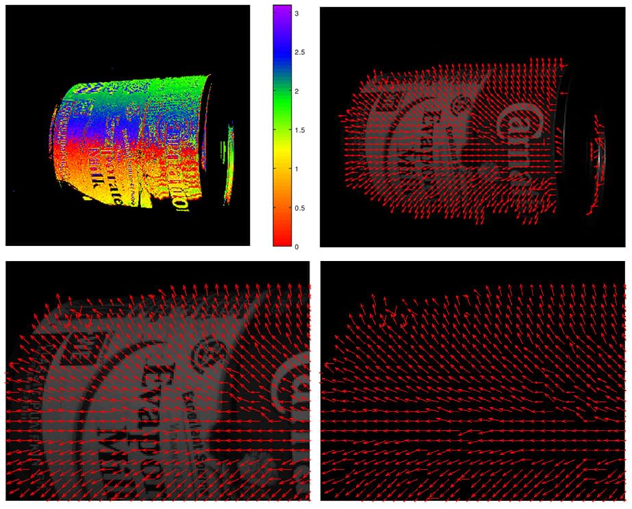
In a can without any deformation, the smooth surface creates surface normals that are more consistent and pointing in the same direction. In both the dented and non-dented examples we can reconstruct depth to create a 3D point cloud.
Example Setup and Code
Step 1. Camera, Lighting and Target Object Setup
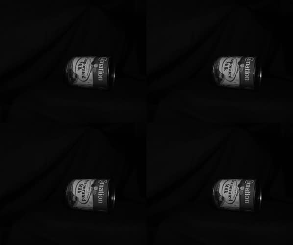
The placement of the camera, light source, and target object should be set at an angle to each other to maximize the results. This takes a level of experimentation but in general, the light source should be placed near the side of the object (e.g. approx. 45deg from the camera). Also, to make it easier to filter out the background, it’s best to use a plain color or dark background.
Step 2. Set camera pixel format to 0°, 45°, 90° and 135° polarized channels
Connect your Triton or Phoenix polarization camera to your PC and launch ArenaView. Select the “PolarizedAngles_0d_45d_90d_135d_Mono8” pixel format to enable on-camera polarization processing based on 0°, 45°, 90° and 135° polarized channels. After choosing the pixel format, capture an image of the target object.
The image taken will be used to estimate surface normals. We’ve also included a sample image in the data folder of Code.zip (download link below) which can be used instead of capturing your own. Your captured image should look similar to the sample image, with 4 images in one (each quadrant representing one of the four polarized angles).
Example image taken using PolarizedAngles_0d_45d_90d_135d_Mono8 pixel format.
Step 3. Download the code files to run in either Matlab or Octave
Please download our zip file containing all the necessary files needed for depth reconstruction from surface normals.
Octave 4.1.1: polar_surface_normal_for_octave_4.1.1.zip (6.5 MB) (For Octave users please load the image processing library.)
MatLab 2020b: polar_surface_normal_for_matlab_2020b.zip (6.5 MB) (For Matlab users the Image Processing Toolbox is required.)
Example using Octave 4.1.1
The main file to run is demo_depth_from_polarization.m. Please note that there exist a few methods that can be used for estimating surface normals. In the provided example code, we use a look-up table approach for the estimation from AoLP. Our look up table approach works only for cylinder objects however other methods and their github links are described along with the code.
Octave users should load the image processing library in Octave before running the code in the next section. This can be done using the console command:
pkg load image
Load and run this file in Octave 4.1.1. The following is a break down of the processes of demo_depth_from_polarization.m
clear allclose all%% Load the captured image of four polarization anglesin_path = 'data/milk_can.tiff';im = imread(in_path);%% Stack the image of four polarization angles into an image of four channels[nrows, ncols] = size(im);im0 = im(1 : nrows/2, 1 : ncols/2);im45 = im(1 : nrows/2, ncols/2 + 1 : end);im90 = im(nrows/2 + 1 : end, 1 : ncols/2);im135 = im(nrows/2 + 1 : end, ncols/2 + 1 : end);images = zeros(nrows/2, ncols/2, 4);images(:, :, 1) = double(im0);images(:, :, 2) = double(im45);images(:, :, 3) = double(im90);images(:, :, 4) = double(im135);nskips = 4; % may work with a smaller image which runs fasterimages = images(1 : nskips : end, 1 : nskips: end, :);%% Assign polarization angles to corresponding channelsangles = [0, 45, 90, 135] * pi / 180;%% May create a mask for a region of interestuse_fg_threshold = true;mask = ones(size(images(:, :, 1)));if ( use_fg_threshold )image_avg = mean(double(images), 3);fg_threshold = 10;mask(image_avg < fg_threshold) = 0;mask(image_avg >=fg_threshold) = 1; % foregroundendmask = logical(mask);figure; imagesc(mask)%% Calculate polarization attributes of the image: dolp, aolp and intensity% credit: PlarizationImage can be found from https://github.com/waps101/depth-from-polarisation[ dolp_est,aolp_est,intensity_est ] = PolarisationImage( images,angles,mask,'linear' );mask(dolp_est < 0.005) = 0; % filter out pixels with very small degree of polarizationfigure; imagesc(aolp_est); colorbar; colormap (rainbow)figure; imagesc(dolp_est); colorbarfigure; imagesc(intensity_est); colormap gray%% Estimate surface normals of the object% This can done with% 1. a Lambertian model; OR% 2. a boundary propagation method; OR% 3. a simple look up table approach given the lighting setup is invariant% The code of methods 1 and 2 can be found in https://github.com/waps101/depth-from-polarisationN = lookup_aolp_cylinder(aolp_est);%[N, height] = Propagation( rho_est,phi_est,mask,n );% We found that a median filter could be used to reduce the noise of the estimated normal vector but it is not a mustN(:,:,1) = imsmooth(N(:,:,1), "Median", [5,5]);N(:,:,2) = imsmooth(N(:,:,2), "Median", [5,5]);N(:,:,3) = imsmooth(N(:,:,3), "Median", [5,5]);%% Depth reconstruction from the derived surface normals% Various methods are described and their codes are included in https://github.com/yqueau/normal_integrationtemp = N(:, :, 3);temp(abs(temp)<1e-5) = nan; % avoid dividing by zero or a very small number. otherwise it will screw up the depth mapN(:, :, 3) = temp;P = -N(:,:,1)./N(:,:,3);Q = -N(:,:,2)./N(:,:,3);P(isnan(P)) = 0;Q(isnan(Q)) = 0;height = DCT_Poisson(P,Q);figure; imagesc(height); colorbarheight(~mask) = nan;figure;surf(height,'EdgeColor','none','FaceColor',[0 0 1],'FaceLighting','gouraud','AmbientStrength',0,'DiffuseStrength',1);axis equal; lightxlabel('x')ylabel('y')zlabel('z')
Conclusion
Analyzing polarization information can be very useful in inspecting an object’s geometrical shape without the need of a traditional 3D camera. Thanks to the Phoenix and Triton polarization cameras, users can obtain AoLP, DoLP, and polarization intensity data from light reflected from an object to estimate surface normals, which then be inspected or be used to reconstruct depth. Deformations in the shape can be identified in surface normals that are very different from their surrounding normals. In the example described above, AoLP data from a metal can is mapped to a Look-Up-Table (LUT) designed to estimate surface normals of cylindrical objects. In addition, various LUTs can be used for different target shapes and users can refer the referenced Githubs for other methods. Finally, polarization data can be used to reconstruct 3D point clouds of the target object (Shape from Polarization). This example shows how it is possible to successfully inspect 3D shape properties of an object using a 2D polarization camera.